Issue 10: How to Read a Loss Exceedance Curve
A step-by-step guide to the chart that connects your analysis to executive decisions"

Issue 10: How to Read a Loss Exceedance Curve
A step-by-step guide to the chart that connects your analysis to executive decisions
In This Issue:
📖 Book Update
🎤 Upcoming Talks
📝 How to Read a Loss Exceedance Curve
❓ Reader Question
📖 Book Update
The finish line is here. From Heatmaps to Histograms is in its final production stages and the release is imminent. I have several book signings planned that I’ll announce in future issues, so there will be plenty of opportunities to connect in person.
If you’ve been thinking about pre-ordering, this is your last window. Pre-orders matter more than most people realize: they signal demand to retailers, influence how the book gets promoted, and give the launch real momentum from day one.
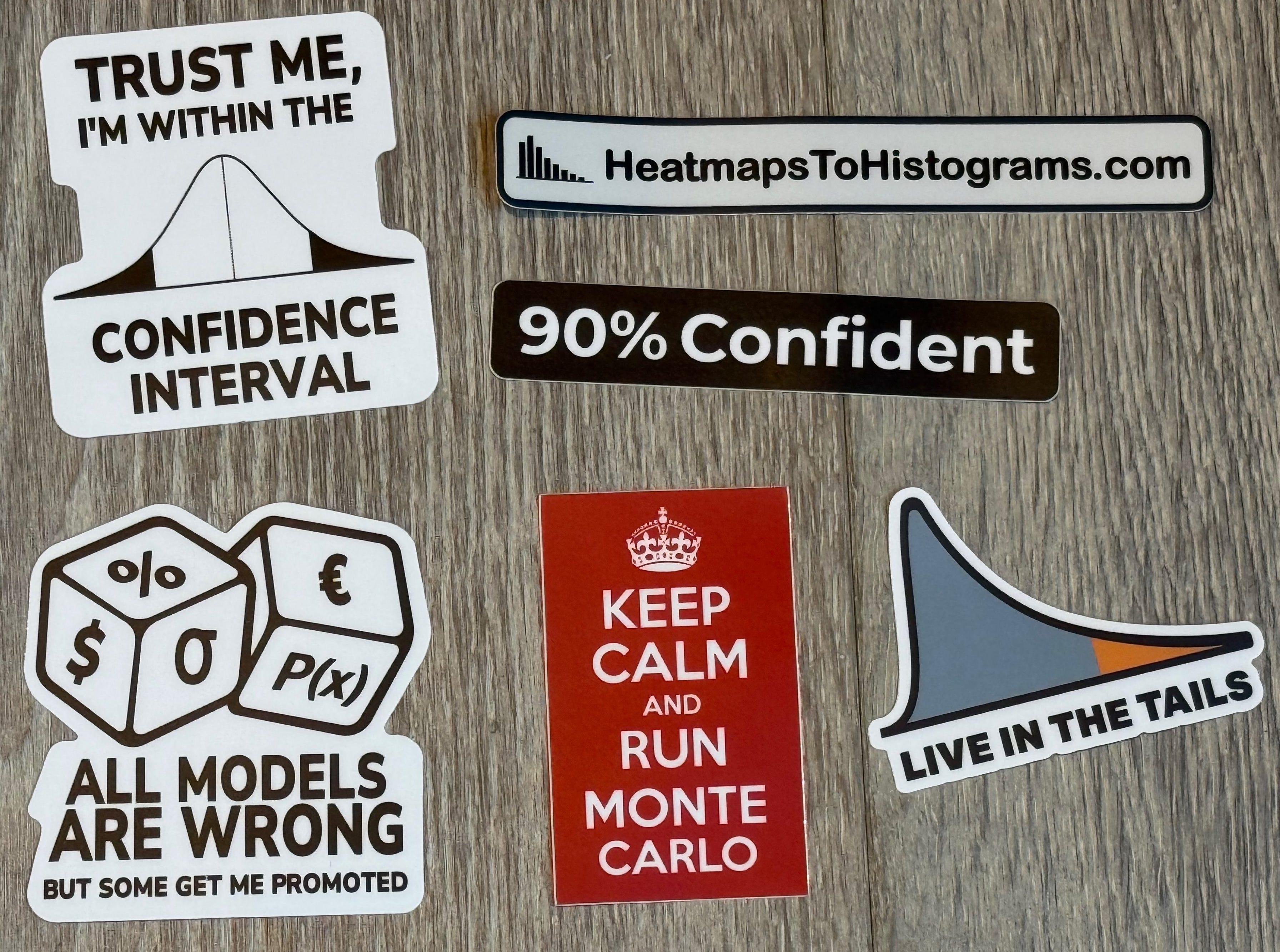
I also have a special offer for newsletter subscribers: if you pre-order and send me a note with your mailing address, I’ll mail you a set of my CRQ stickers. International mailing addresses are perfectly fine.
🔗 Pre-order on Amazon | 🔗 Book website
🎤 Upcoming Talks
March 24, 2026 — “The Future of Cyber Risk Intelligence” FAIR Institute Seminar at RSAC 2026, San Francisco
I’m closing out the FAIR Institute’s seminar at RSA with a session on the shift from backward-looking risk reporting to forward-looking risk intelligence. The FAIR seminar is always one of the best events of RSA week, and I’d encourage anyone attending the conference to make time for it.
April 21, 2026 — “Did We Solve the Data Problem? Judgment, Beliefs, and Risk in the AI Age” SIRAcon 2026 — Keynote
I’m keynoting SIRAcon this year with a talk on why the real bottleneck in risk quantification was never data, it was judgment, and why AI makes that distinction more important than ever. SIRAcon remains my favorite conference because it is model-neutral, vendor-neutral, and entirely dedicated to advancing risk practices.
📝 How to Read a Loss Exceedance Curve
I’ve shown the same chart to hundreds of people across different fields. Finance teams nod and start asking questions about the tail. MBAs recognize it from business school, and engineers start interpreting it and reading their interpretation back to me before I finish explaining the axes. When I show the exact same chart to information security professionals, I usually get blank stares.
MBAs recognize it from business school, and engineers start interpreting it and reading their interpretation back to me before I finish explaining the axes.
The chart is a loss exceedance curve, and I’d argue it’s one of the most important visualizations in cyber risk quantification. It’s also the one that confuses security people the most, which is a problem because it’s the chart that executives already think in. They’ve seen it in insurance models, in business forecasts, in scenario planning. They just haven’t seen it come from a security team.
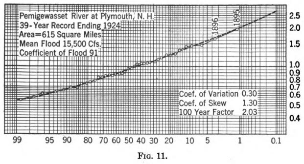
This might reframe how you feel about this chart if it’s unfamiliar to you: it’s not new. The exceedance curve has been around for over a century. Hydrologists were using it to model flood risk long before anyone was quantifying cyber threats, plotting the probability that a river would exceed a given height in a given year. Insurance companies have relied on it for decades to price policies and set reserves. Weather forecasters, structural engineers, and financial analysts all use the same underlying concept. The x-axis represents a magnitude of something (water height, wind speed, financial loss) and the y-axis represents the probability of exceeding that magnitude.
Cyber risk quantification didn’t invent this visualization. It borrowed a proven tool from fields that have been reasoning about uncertainty far longer than information security has existed. If the chart feels foreign to you, that’s on us, not on the chart. Security has spent decades trapped in qualitative frameworks, heat maps and red-yellow-green dashboards, and we never learned how other disciplines communicate risk along the way.
This issue is my attempt to fix that, at least for this one chart. It’s not complicated. It just hasn’t been taught well to security practitioners.
Start with the Shape: The Histogram
Before you can understand a loss exceedance curve, you need to know what it’s built from.
When you run a quantitative risk assessment using a framework like FAIR, the engine underneath is a Monte Carlo simulation. You provide estimated ranges that define probability distributions for your inputs, and the simulation samples from those distributions across thousands of trials, sometimes 10,000, sometimes 50,000 or more. A frequency distribution might be centered between 1 and 4 times per year, and a loss magnitude distribution might span $50,000 to $500,000. Each trial represents one possible version of next year. Most simulated years are unremarkable, a few are catastrophic, and the spread between those outcomes is where the interesting information lives.
The first way to visualize those results is a histogram. It groups the simulated outcomes into bins and displays them as a bar chart. The x-axis shows loss amounts and the y-axis shows the percentage of simulations that landed in each range.
The histogram shows you the shape of risk: where most losses cluster, how wide the spread is, and whether there’s a long tail of expensive outcomes stretching to the right. A narrow peak means the losses are fairly predictable. A wide spread or a long tail means there’s real uncertainty about how bad things could get, and that uncertainty demands different planning than a tight distribution does.
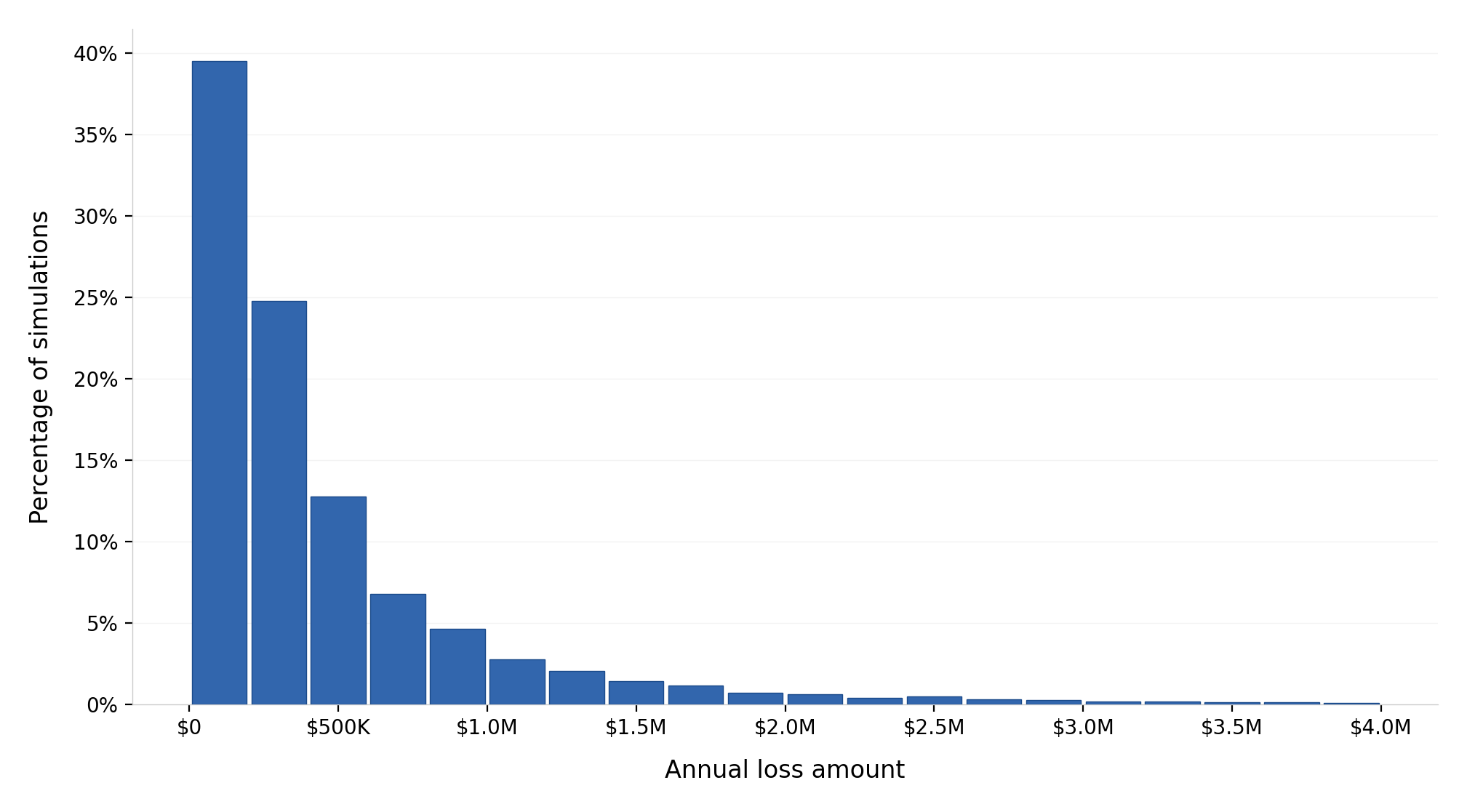
The y-axis on a histogram shows the percentage of simulations that produced different loss amounts. It does not show the probability of an incident happening. Think of each bar as answering the question “if something bad happens, here’s how bad it’s likely to be.” The frequency of the event itself is already baked into the annual loss exposure calculation.
The histogram is useful, though it has a limitation: it doesn’t answer the question that executives ask most often, which is “what are the chances we lose more than $X?” For that, you need the loss exceedance curve.
How a Loss Exceedance Curve Is Built
The math behind a loss exceedance curve is simpler than most people expect. If you can sort a column of numbers and do basic division, you already know how this works.
Imagine your Monte Carlo simulation produced 50,000 results, and they’re sitting in a spreadsheet column, one per row. Each number represents the total annual loss from one simulated year. Some are zero, some are modest, and a few are enormous.
To build the curve, you conceptually sort those 50,000 results from smallest to largest. Then, for any dollar amount you want to examine, you count how many of the 50,000 results exceeded that amount and divide by 50,000. That gives you the exceedance probability for that dollar amount.
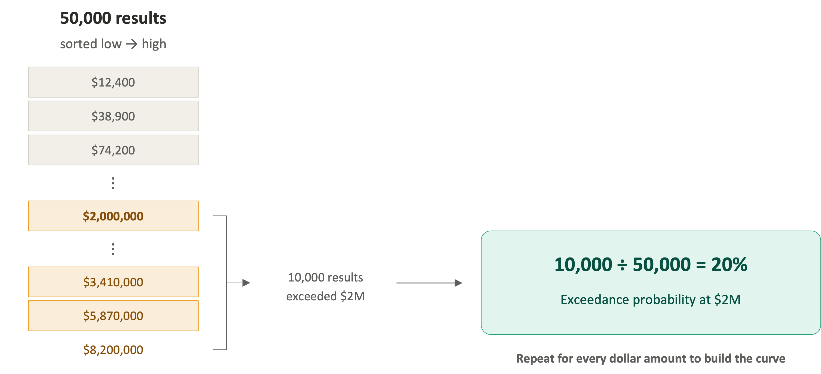
If 10,000 of your 50,000 results exceeded $2 million, the exceedance probability at $2 million is 10,000 divided by 50,000, which is 20%. If 2,500 results exceeded $5 million, the exceedance probability at $5 million is 5%. Plot every dollar amount against its exceedance probability, and you get the curve.
That’s the entire construction. Just “what fraction of my simulated outcomes were worse than this amount?” repeated across every dollar value on the x-axis. The curve slopes downward from left to right because fewer and fewer simulations produce extreme outcomes as you move toward higher loss amounts.
I often spend extra time on the construction with skeptics because people trust a chart more when they understand what’s underneath it. When you can explain to someone that the curve is built from 50,000 simulated scenarios and each point represents a simple fraction, you’re building trust in not only the chart, but the underlying methodology and process.
One caveat: the curve will faithfully reflect whatever you feed it. If your input distributions are poorly reasoned or pulled from thin air, the LEC will produce a polished, confident-looking result that points you in the wrong direction. The visualization doesn’t validate the analysis; that’s something you still need to do.
I built an interactive tool for the book’s companion site that lets you run through this entire construction yourself, from setting inputs to watching the histogram transform into an exceedance curve. Try it here.
What the Loss Exceedance Curve Shows
The histogram and the LEC are built from the same simulation data, though they answer different questions. The histogram answers “what does the spread of outcomes look like?” The LEC answers “what are the chances we lose more than a given amount?”
I call the LEC the “What Are the Chances?” chart because that’s the question it answers in every conversation where it matters. What are the chances we lose more than $10 million? What are the chances losses exceed our insurance coverage? What are the chances this risk is bigger than the project we’re considering? Every one of those questions maps to a single point on the curve.
I call it the “What Are the Chances?” chart because that’s the question it answers in every conversation where it matters.
This is why executives respond to it immediately. They’re accustomed to reasoning in terms of exposure and probability because every other risk function in the organization already communicates this way. Finance, insurance, and operational risk all speak this language, and security has been the holdout, bringing heat maps to a conversation where everyone else brings probabilities. The LEC gets you a seat at that table.
How to Read It: Three Steps
Reading a loss exceedance curve takes three steps.
The y-axis shows probabilities, running from 0% at the bottom to 100% at the top. The x-axis shows dollar amounts, increasing from left to right. The curve itself shows the probability of losses exceeding any given dollar amount.
Step 1. Find your dollar amount of interest on the x-axis. Let’s use $35 million as our example.
Step 2. Move straight up from that point until you hit the curve.
Step 3. Move horizontally to the left and read the probability on the y-axis. In this example, you’d land at approximately 20%.
That gives you: “There is a 20% chance that losses will exceed $35 million.”
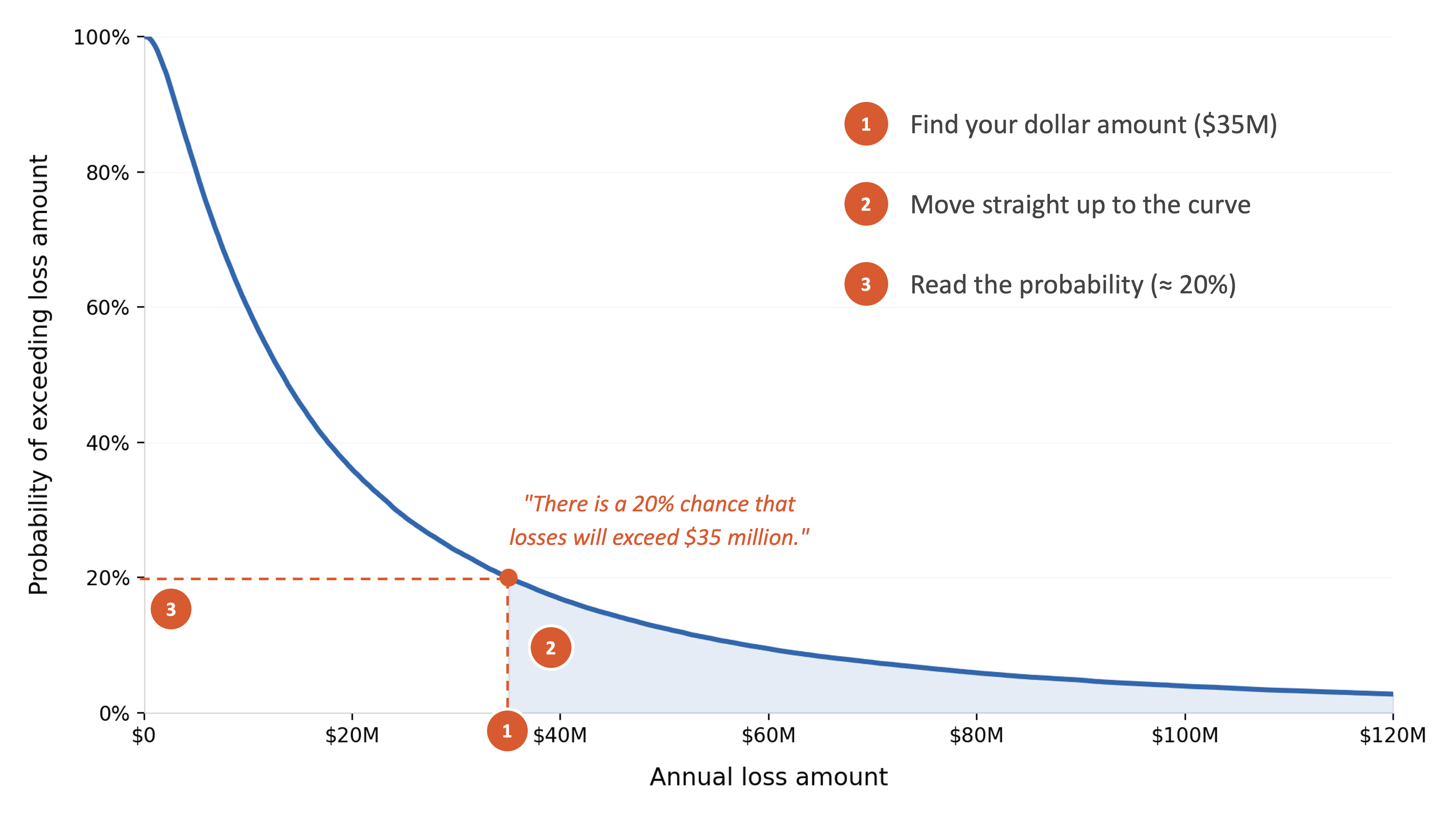
If you look at the shaded area above and to the right of the $35 million mark, that region represents the 20% probability zone, all the outcomes where losses exceed $35 million. The larger the shaded area at any given point, the higher the probability of exceeding that loss amount. As you move further to the right toward larger losses, the shaded area shrinks because fewer and fewer simulated outcomes reach those extremes.
The Y-Axis Trap
Misunderstanding the Y-axis is the most common mistake I encounter when people are new to the LEC.
The y-axis does not show how often incidents occur. It shows the probability that losses exceed a particular dollar amount. The simulation already accounts for how often events happen; that’s built into the annual loss exposure before the curve is ever drawn.
The confusion makes sense when you think about where security professionals come from. We’re trained to think in terms of “will an attack happen?” The LEC answers a different question: “if something bad happens, how bad could it get?” If you mix those two up, the y-axis will mislead you.
Loss Exceedance Statements
I always accompany a loss exceedance curve with written statements that serve as a voiceover for people who aren’t comfortable reading probability graphs.
The format goes something like this:
“There is a 20% chance that losses will exceed $2 million.”
“We have a 50/50 chance of losses exceeding $500,000.”
“There is only a 5% chance we would see losses above $8 million.”
Each statement is a single point on the curve translated into plain language. You pick the dollar amounts that matter to your audience, read the corresponding probabilities, and write the sentences.
Here’s the presentation technique that I’ve found lands well: start with the loss exceedance statements, then show the curve. When you lead with the narrative, you prime your audience so they know what to look for before the chart appears on screen. They understand what the axes mean, they’re oriented, and the visual confirms what they’ve already absorbed. I’ve been doing it this way for years, and the difference in how people engage is night and day compared to showing the chart cold and trying to explain it after the fact.
Anchoring the Curve to Real Decisions
You should not pick an arbitrary dollar amount to point out to audiences. Pick amounts that matter to your organization. I use five anchors regularly.
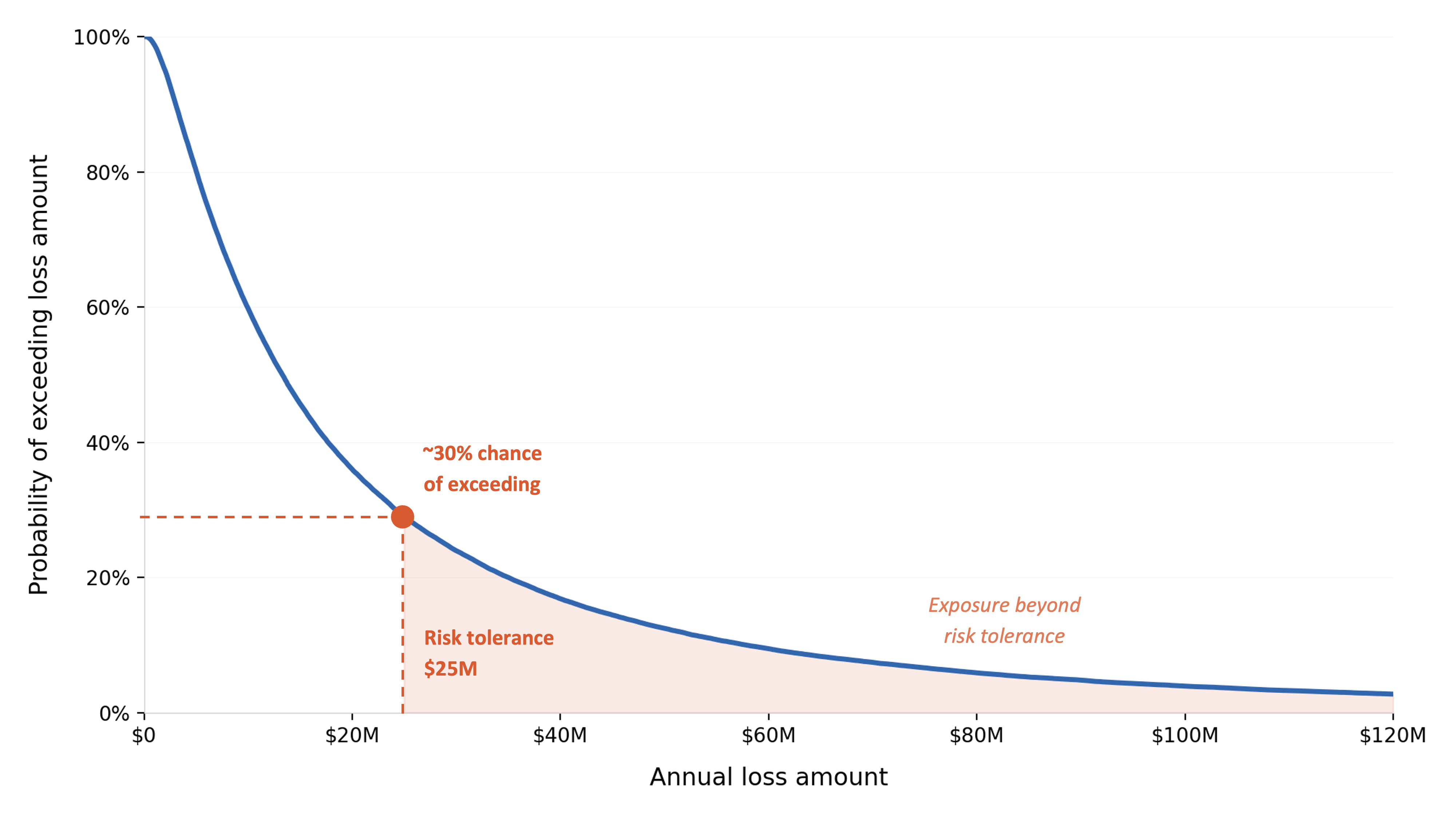
Risk tolerance. Ask your board or CFO what the maximum loss the organization can absorb before it threatens operations. Use that number as your primary anchor point on the curve. If there’s a 30% chance of exceeding your stated risk tolerance, that’s a conversation worth having.
Cyber insurance limit. Losses beyond the policy limit are uninsured, and the organization bears the full impact. Plot your insurance limit on the curve and read the exceedance probability. Keep in mind that exclusions and sub-limits for things like ransomware or regulatory fines may reduce the effective coverage, so the real exposure might start earlier than the headline policy number suggests.
Budget thresholds. Compare the curve to your contingency or emergency reserves. If there’s a 60% chance of exceeding those reserves, your planning needs attention regardless of what the risk appetite statement says.
SEC materiality. For public companies, ask legal at what loss level disclosure would likely be required. There’s no fixed dollar rule since materiality depends on context, though establishing a working threshold makes the curve actionable for your compliance team.
Project costs. Compare loss probabilities to the cost of proposed security investments. If there’s a 40% chance of losses exceeding the cost of a $3 million project, the investment starts to look justified in a way that a heat map could never communicate.
Once you start overlaying these thresholds on the curve, the conversation changes. You’re answering questions your stakeholders already have, using numbers they already care about, and in my experience that’s the moment the LEC earns its place in every presentation you give.
Closing
The loss exceedance curve isn’t exotic. Hydrologists, insurers, and financial analysts have relied on it for over a century because it answers the question that matters most when you’re making decisions under uncertainty: what are the chances things get worse than this?
Cyber risk quantification adopted it for the same reason. If this chart is new to you, you’re in good company. Most security professionals never encountered it because our field spent decades in qualitative frameworks that didn’t require it. Once you learn to read it, the way your executives engage with your work will look very different.
🔗 Interactive tool: Build and read a Loss Exceedance Curve
❓ Reader Question
“I’m a security analyst thinking about moving into risk quantification. Is it worth getting the FAIR certification, or should I just start doing the work?”
Both, but start with the work. The certification will make more sense after you’ve worked on a few real assessments, because the concepts stick differently when you’ve already felt the pain of scoping a scenario or arguing over a frequency estimate. If you study for the exam first with no practical context, it reads like theory. If you do two or three assessments first, even rough ones, the material reads like answers to questions you already have.
That said, the FAIR certification is worth pursuing. It gives you a shared vocabulary and understanding with other practitioners, it signals to hiring managers that you’re serious about the discipline, and the study process will tighten your understanding of the taxonomy in ways that doing the work alone won’t. It’s not expensive, and it’s not a months-long commitment.
The bigger career advice is this: build a portfolio of work product. Run an assessment, document it, present the results internally, and refine your approach based on the questions you get. Three completed assessments with clear write-ups will do more for your career trajectory than any credential on its own.
✉️ Contact
Have a question about this, or anything else? Here’s how to reach me:
Reply to this newsletter if reading via email
Comment below
Connect with me on LinkedIn
🌐 Elsewhere
I share shorter thoughts on risk, metrics, and decision-making on LinkedIn.
Book updates, chapter summaries, tools, and downloads are at www.heatmapstohistograms.com
My longer-form essays and older writing live at www.tonym-v.com
❤️ How You Can Help
✅ Tell me what topics you want covered: beginner, advanced, tools, AI use, anything ✅ Forward this to a colleague who’s curious about CRQ
✅ Click the ❤️ or comment if you found this useful
If someone forwarded this to you, please subscribe to get future issues.
Thanks for reading.
—Tony